Do you have individual column sections and angled wall geometries, and need punching shear design for them?
No problem. In RFEM 6, you can perform punching shear design not only for rectangular and circular sections, but for any cross-section shape.
- Design of five types of seismic force-resisting systems (SFRS) includes Special Moment Frame (SMF), Intermediate Moment Frame (IMF), Ordinary Moment Frame (OMF), Ordinary Concentrically Braced Frame (OCBF), and Special Concentrically Braced Frame (SCBF)
- Ductility check of the width-to thickness ratios for webs and flanges
- Calculation of the required strength and stiffness for stability bracing of beams
- Calculation of the maximum spacing for stability bracing of beams
- Calculation of the required strength at hinge locations for stability bracing of beams
- Calculation of the column required strength with the option to neglect all bending moments, shear, and torsion for overstrength limit state
- Design check of column and brace slenderness ratios
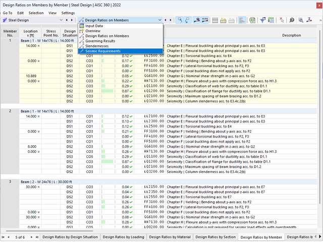
The seismic design result is categorized into two sections: member requirements and connection requirements.
The "Seismic Requirements" include the Required Flexural Strength and the Required Shear Strength of the beam-to-column connection for moment frames. They are listed in the ‘Moment Frame Connection by Member’ tab. For braced frames, the Required Connection Tensile Strength and the Required Connection Compressive Strength of the brace are listed in the ‘Brace Connection by Member’ tab.
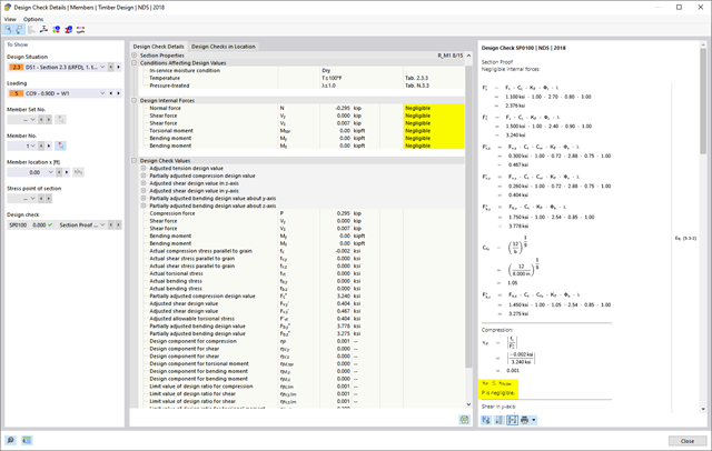
The program provides the performed design checks in tables. The design check details clearly display the formulas and references to the standard.

The building model is calculated in two phases:
- Global 3D calculation of the global model, where the slabs are modeled as a rigid plane (diaphragm) or as a bending plate
- Local 2D calculation of the individual floors
After the calculation, the results of the columns and walls from the 3D calculation and the results of the slabs from the 2D calculation are combined in a single model. This means that there is no need to switch between the 3D model and the individual 2D models of the slabs. The user only works with one model, saves valuable time, and avoids possible errors in the manual data exchange between the 3D model and the individual 2D ceiling models.
The vertical surfaces in the model can be divided into shear walls and opening lintels. The program automatically generates internal result members from these wall objects, so they can be designed as members according to any standard in the Concrete Design add-on.
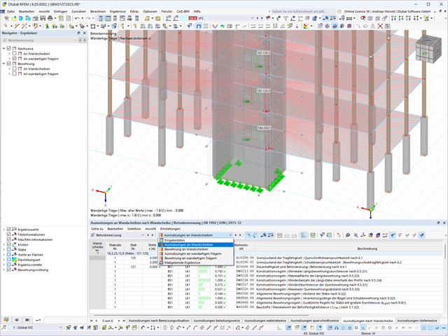
Shear walls and deep beams of a building model are available as independent objects in the design add-ons. This allows for faster filtering of the objects in results, as well as better documentation in the printout report.
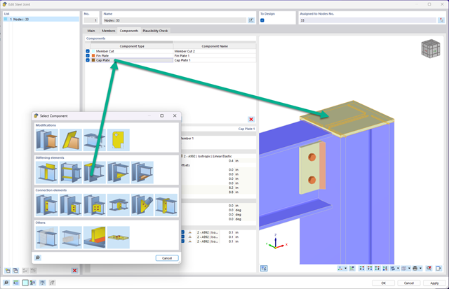
You can now insert a cap plate in steel joints with only a few clicks. You can enter the data using the known definition types "Offsets" or "Dimensions and Position". By specifying a reference member and the cutting plane, it is also possible to omit the Member Section component.
This component allows you to easily model cap plates on column ends, for example.
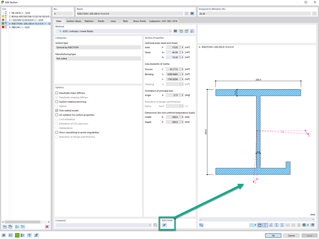
You can open the cross-sections in RSECTION using a direct connection, modify them there, and transfer them back to RFEM/RSTAB. Both RSECTION cross-sections and library cross-sections, with the exception of elliptical, semi-elliptical and virtual joists, can be opened and modified directly in RSECTION by clicking a button.
For example, you can thus adjust the reinforcement layout of user-defined RSECTION cross-sections directly in a local RSECTION environment in RFEM/RSTAB. This feature is currently only available for cross-sections with a uniform distribution type. The shear and longitudinal reinforcement defined for library cross-sections is not imported into RSECTION.
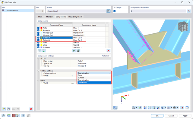
You can use the "Plate Cut" component to cut plates (for example, gusset plates, fin plates, and so on). There are various cutting methods available:
- Plane: The cut is performed on the closest surface to the reference plate.
- Surface: Only the intersecting parts of plates are cut.
- Bounding Box: The outermost dimension consisting of width and height is cut out of the plate as a rectangle.
- Convex Envelope: The outer hull of the cross-section is used for the plate cut. If there are fillets at the corner nodes of the cross-section, the cut is adapted to them.
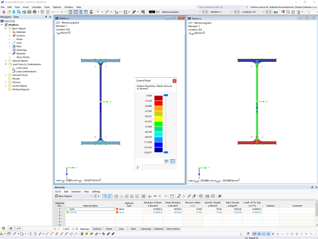
Within the "Plastic capacity design | Simplex Method" in RSECTION, the simultaneous variation of shear stresses over the cross-sectional area is performed in addition to the variation of axial stresses. This extended form of analysis allows you to use redistribution reserves, especially for the cross-sections subjected to shear loading, thus loading the cross-sections even more efficiently.
Go to Explanatory Video
Several modeling tools are available for elements in building models:
- Vertical line
- Column
- Wall
- Beam
- Rectangular floor
- Polygonal floor
- Rectangular floor opening
- Polygonal floor opening
This feature allows you to define the element on the ground plane (for example, with a background layer) with the associated multiple element creation in space.
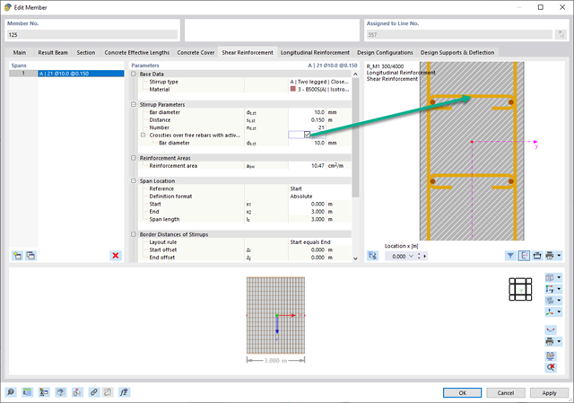
In the "Shear Reinforcement" tab, you can select the option "Cross-ties over free rebars with active selection in graphic". It allows you to arrange additional cross-ties on free rebars of the longitudinal reinforcement.
You can activate or deactivate the position of the cross-ties in the Info Graphic. The cross-ties are applied for the ultimate limit state design and the structural design checks. They are available for the design according to EN 1992‑1‑1.
Go to Explanatory Video
Using the "Load Transfer Only" story type, you can consider slabs without stiffness effect in and out of the plane in the Building Model add-on. This element type collects the loads on the slab and transfers them to the supporting elements of a 3D model. Thus, you can simulate secondary components, such as grillage and similar load distribution elements, without any further effect in the 3D model.
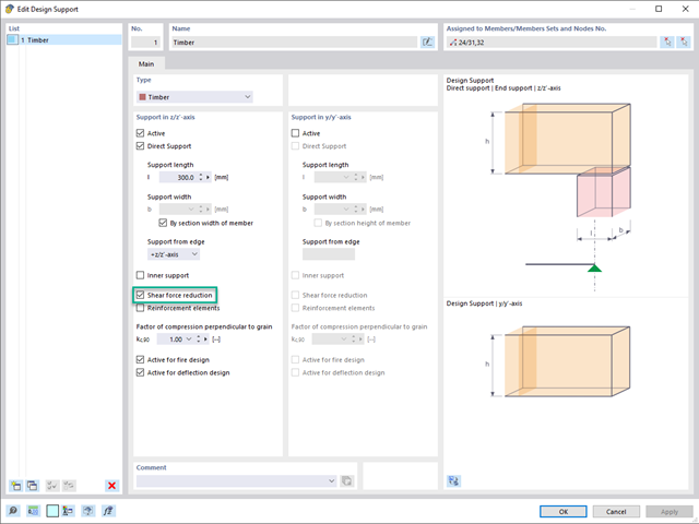
For design supports, you can take into account a shear force reduction. This allows you to perform the shear design with the governing shear force at a distance of the beam height from the support edge.
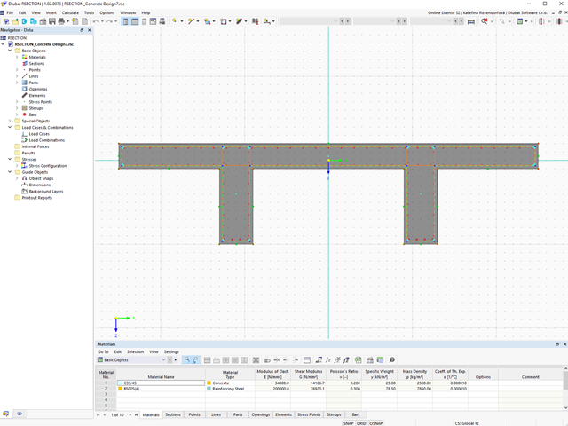
In the Concrete Design add-on, you can design any RSECTION cross-section. Define the concrete cover, shear force, and longitudinal reinforcement directly in RSECTION.
After importing the reinforced RSECTION cross-section into RFEM 6 or RSTAB 9, you can use it for design in the Concrete Design add-on.
Go to Explanatory Video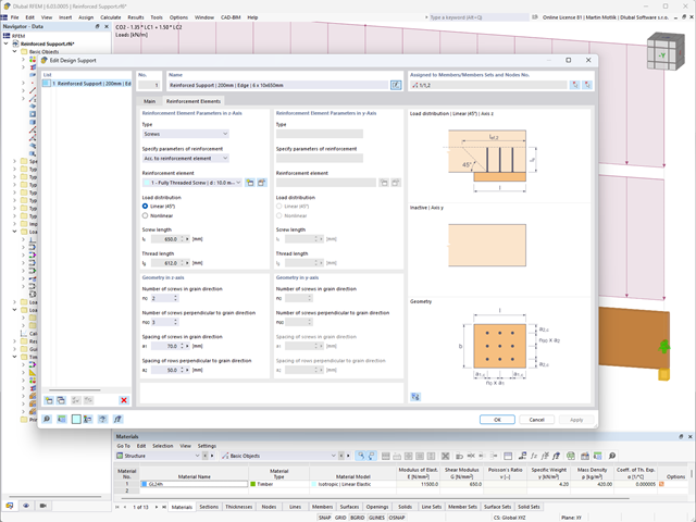
Did you know? In the Design Supports, you can now define fully threaded screws as transversal compression stiffening elements for the "Compression Perpendicular to Grain" design. In this case, the pressing-in and buckling of the bolts is analyzed.
Moreover, the design shear resistance is checked in the plane of the screw tip. The angle of dispersal can be considered as linear under 45° or nonlinear (according to Bejtka, I. (2005). Verstärkung von Bauteilen aus holz mit vollgewindeschrauben. KIT Scientific Publishing.).
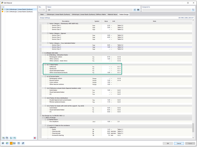
For timber surfaces with the "Constant" thickness type, the crack factor kcr and thus the negative influence of cracks on the shear capacity is taken into account.
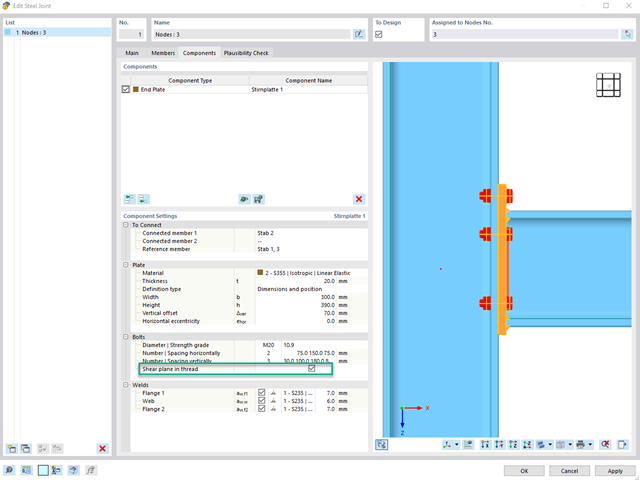
To determine the shear resistance of bolts, you can use the Steel Joints add-on to specify whether there is a shaft or a thread in the shear plane.
Go to Explanatory Video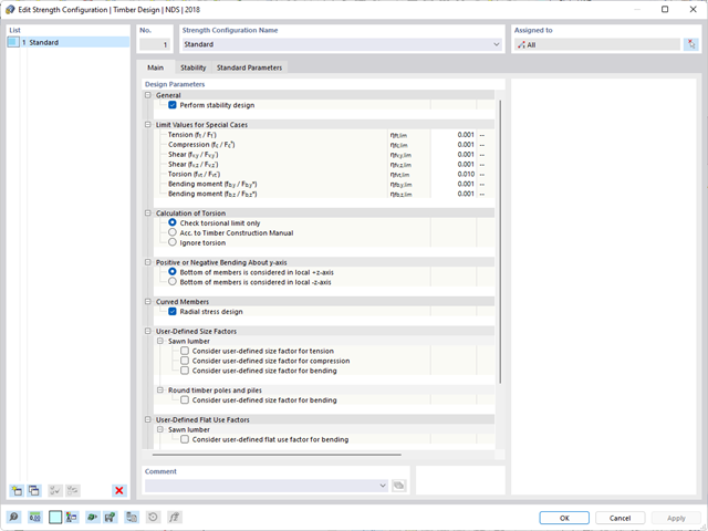
Is there torsion? In this case, you can decide how to perform the design. You have the following options:
- Allow further design if shear stress due to torsion does not exceed limit value
- Design according to Timber Construction Manual, 4.6
- Ignoring torsion
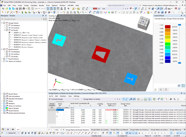
Do you work with the structural components consisting of slabs? In that case, you have to perform the shear force design with the requirements of punching shear design, for example, according to 6.4, EN 1992‑1‑1. In addition to floor slabs, you can also design foundation slabs in this way.
In the Ultimate Configuration for concrete design, you can define the punching design parameters for the selected nodes.
.png?mw=640&hash=55038d2a1591f62179796666cb9b2fede0274e19)
A graphical and tabular output of the results for deformations, stresses, and strains helps you when determining the soil solids. To achieve this, use the special filter criteria for targeted selection of results.
The program doesn't leave you alone with the results. If you want to graphically evaluate the results in the soil solids, you can use the guide objects. For example, you can define clipping planes. This allows you to view the corresponding results in any plane of the soil solid.
And not just that. The utilization of result sections and clipping boxes facilitates the precise graphical analysis of the soil solid.
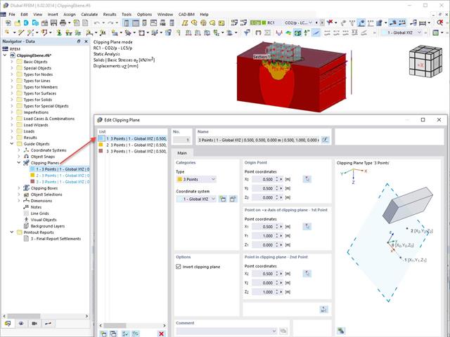
This feature also contributes to the clearly-arranged display of your results. Clipping planes are intersecting planes that you can place freely throughout the model. The zone in front of or behind the plane is consequently hidden in the display. This way, you can clearly and simply show the results in an intersection or a solid, for example.
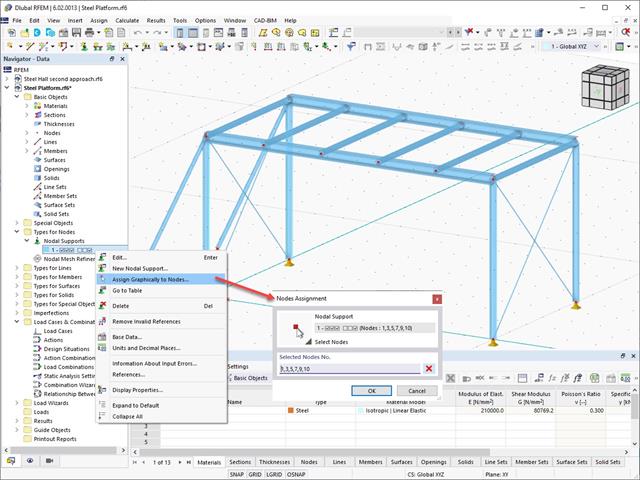
The object types listed below can be graphically assigned to the elements of the structure modeled in the program.
- Nodal supports
- Member shear panels
- Local reductions of member cross-sections
- Member transverse stiffeners
- Member longitudinal welds
- Effective lengths
- Boundary conditions
- Line supports
- Loads
- Member support
- Punching reinforcements
- Mesh refinements
- Surface reinforcements
- Surface results adjustments
- Surface support
- Service classes
- Imperfections
- Design of tension, compression, bending, shear, torsion, and combined internal forces
- Consideration of a notch
- Design of compression perpendicular to the grain on the end and intermediate supports with (EC 5) and without reinforcement elements (fully threaded screws)
- Optional shear force reduction at the support (see the Product Feature)
- Design of curved and tapered members
- Consideration of higher strengths for similar components that are close together (factor ksys according to EN 1995‑1‑1, 6.6(1)-(3))
- Option to increase shear resistance for softwood timber according to DIN EN 1995‑1‑1:NA NDP to 6.1.7(2)
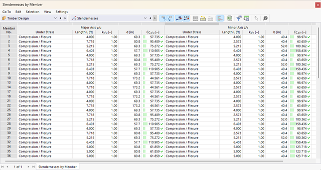
- Stability analyses for flexural buckling, torsional buckling, and flexural-torsional buckling under compression
- Import of the effective lengths from the calculation using the Structure Stability add-on
- Graphical input and check of the defined nodal supports and effective lengths for stability analysis
- Determination of the equivalent member lengths for tapered members
- Consideration of Lateral-Torsional Bracing Position
- Lateral-torsional buckling analysis of the structural components subjected to moment loading
- Depending on the standard, a choice between user-defined input of Mcr, analytical method from the standard, and use of internal eigenvalue solver
- Consideration of a shear panel and a rotational restraint when using the eigenvalue solver
- Graphical display of a mode shape if the eigenvalue solver was used
- Stability analysis of structural components with the combined compression and bending stress, depending on the design standard
- Comprehensible calculation of all necessary coefficients, such as the factors for considering moment distribution or interaction factors
- Alternative consideration of all effects for the stability analysis when determining internal forces in RFEM/RSTAB (second-order analysis, imperfections, stiffness reduction, possibly in combination with the Torsional Warping (7 DOF) add-on)
.png?mw=640&hash=342149908caead326e60e26a2b5d05f7f46825cb)
Are you familiar with the Tsai-Wu material model? It combines plastic and orthotropic properties, which allows for special modeling of materials with anisotropic characteristics, such as fiber-reinforced plastics or timber.
If the material is plastified, the stresses remain constant. The redistribution is carried out according to the stiffnesses available in the individual directions. The elastic area corresponds to the Orthotropic | Linear Elastic (Solids) material model. For the plastic area, the yielding according to Tsai-Wu applies:
All strengths are defined positively. You can imagine the stress criterion as an elliptical surface within a six-dimensional space of stresses. If one of the three stress components is applied as a constant value, the surface can be projected onto a three-dimensional stress space.
If the value for fy(σ), according to the Tsai-Wu equation, plane stress condition, is smaller than 1, the stresses are in the elastic zone. The plastic area is reached as soon as fy (σ) = 1; values greater than 1 are not allowed. The model behavior is ideal-plastic, which means there is no stiffening.

Did you know? In contrast to other material models, the stress-strain diagram for this material model is not antimetric to the origin. You can use this material model to simulate the behavior of steel fiber-reinforced concrete, for example. Find detailed information about modeling steel fiber-reinforced concrete in the technical article about Determining the material properties of steel-fiber-reinforced concrete.
In this material model, the isotropic stiffness is reduced with a scalar damage parameter. This damage parameter is determined from the stress curve defined in the Diagram. The direction of the principal stresses is not taken into account. Rather, the damage occurs in the direction of the equivalent strain, which also covers the third direction perpendicular to the plane. The tension and compression area of the stress tensor is treated separately. In this case, different damage parameters apply.
The "Reference element size" controls how the strain in the crack area is scaled to the length of the element. With the default value zero, no scaling is performed. Thus, the material behavior of the steel fiber concrete is modeled realistically.
Find more information about the theoretical background of the "Isotropic Damage" material model in the technical article describing the Nonlinear Material Model Damage.
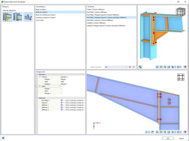
- Many predefined components available for easy input of typical connection situations (for example, end plates, cleats, fin plates)
- Universally applicable basic components (plates, welds, bolts, auxiliary planes) for entering complex connection situations
- Graphical display of the connection geometry that is updated in parallel with the input
- The Steel Joints Template included in the Add-on allows you to select from several connection types and, when selected, is applied to your model
- In the Template, there are connections from 3 general categories: Rigid, Pinned, Truss
- Automatic adaptation of the connection geometry, even if the members are subsequently edited, due to the relative relation of the components to each other
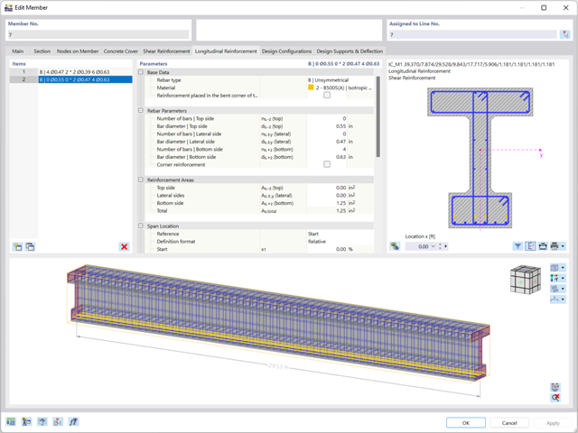
You can specify the shear and longitudinal reinforcement individually for each member. In this case, there are various templates available for entering the reinforcement.

Did you know that you can also display the moment-axial force interaction diagrams (M‑N diagrams) graphically? This allows you to display the cross-section resistance in the case of an interaction of a bending moment and an axial force. In addition to the interaction diagrams related to the cross-section axes (My‑N diagram and Mz‑N diagram), you can also generate an individual moment vector to create an Mres‑N interaction diagram. You can display the section plane of the M‑N diagrams in the 3D interaction diagram. The program displays the corresponding value pairs of the ultimate limit state in a table. The table is dynamically linked to the diagram so that the selected limit point is also displayed in the diagram.

Do you want to determine the biaxial bending resistance of a reinforced concrete cross-section? For this, you have to activate a moment-moment interaction diagram (My-Mz diagram) first. This My-Mz diagram represents a horizontal section through the three-dimensional diagram for the specified axial force N. Due to the coupling to the 3D interaction diagram, you can also visualize the section plane there.